【Python】活性化関数を描画する
概要
Deep Learningのニューロンで使用する活性化関数としてステップ関数、シグモイド関数、ReLu関数などがあります。
素人なので、あまり詳しくはないですが、よく使われるのはReLu関数らしいです。
今回はこの活性化関数とその微分をpythonで描画して実際にどんな特性があるのか可視化してみたいと思います。
使用するライブラリ
- numpy
- matplotlib.pyplot
ステップ関数
import numpy as np
import matplotlib.pyplot as plt

#関数定義
def step(x):
    return 1.0*(x>=0)

#ステップ関数入出力データ作成
x = np.linspace(-1,1,500)
y = step(x)

#描画
fig = plt.figure()
ax = fig.add_subplot(111)
ax.plot(x,y)
plt.show()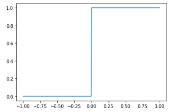
シグモイド関数
#sigmoid関数
def sigmoid(x):
    return 1/(1+np.exp(-x))

#sigmoidの導関数
def derivative_sigmoid(x):
    return sigmoid(x)*(1-sigmoid(x))

#sigmoid関数入出力データ作成
x = np.linspace(-5,5)
y = sigmoid(x)

#描画
fig = plt.figure()
ax = fig.add_subplot(211)
ax.plot(x,y)
plt.title('sigmoid')

#sigmoidの導関数の出力データ作成
y = derivative_sigmoid(x)

#描画
ax = fig.add_subplot(212)
ax.plot(x,y)
plt.title('derivative sigmoid')

#グラフ間隔調整
plt.subplots_adjust(wspace=0.4, hspace=0.6)
plt.show()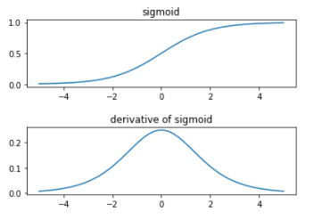
tahn関数
#tanh関数の入出力データ作成
x = np.linspace(-5,5)
y = np.tanh(x)

#描画
fig = plt.figure()
ax = fig.add_subplot(211)
ax.plot(x,y)
plt.title('tanh')

#tanhの導関数
def derivative_tanh(x):
    return 4/((np.exp(x)+np.exp(-x))**2)

#tanh導関数の出力データ作成
y = derivative_tanh(x)

#描画
fig = plt.figure()
ax = fig.add_subplot(212)
ax.plot(x,y)
plt.title('derivative tanh')

plt.show()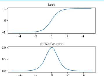
ReLu関数
#ReLu関数定義
def relu(x):
    return x*(x>=0)

#ReLu関数の入出力データ作成
x = np.linspace(-5,5,500)
y = relu(x)

#描画
fig = plt.figure()
ax = fig.add_subplot(211)
ax.plot(x,y)
plt.title('ReLu')

#ReLuの導関数定義
def derivative_relu(x):
    return 1*(x>=0)

#ReLu導関数の出力データ作成
y = derivative_relu(x)

#描画
fig = plt.figure()
ax = fig.add_subplot(212)
ax.plot(x,y)
plt.title('derivative ReLu')

plt.show()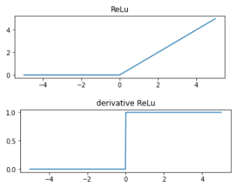
Leaky ReLu関数
#Leaky ReLu関数の定義
def leaky_relu(x):
    return np.where(x < 0,0.01*x,x)

#Leaky ReLu関数の入出力データ作成
x = np.linspace(-5,5,500)
y = leaky_relu(x)

#描画
fig = plt.figure()
ax = fig.add_subplot(111)
ax.plot(x,y)
plt.title('Leaky ReLu')

#Leaky ReLu導関数の定義
def derivative_leaky_relu(x):
    return np.where(x < 0,0.01,1)

#導関数の出力データ作成
y = derivative_leaky_relu(x)

#描画
fig = plt.figure()
ax = fig.add_subplot(111)
ax.plot(x,y)
plt.title('derivative Leaky ReLu')

plt.show()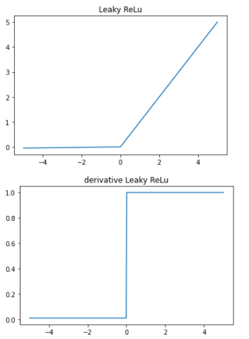
まとめ
シグモイド関数は導関数の値が最大でも0.25程度のため、誤差逆伝播したときに勾配消失が起きやすい。
それに対してtanhやReLuは最大1.0なのでsigmoidより使いやすいらしい。