【keras】preprocessing.timeseries_dataset_from_arrayの使い方
概要
時系列のディープラーニングに便利なkeras(tensorflow)のpreprocessing.timesiereis_dataset_from_arrayというメソッドがあるので、サンプルデータを使って使い方を覚えようと思います。
このメソッドは簡単に言うと時系列データに対しサンプリングレート、シーケンス長さ、ストライド、バッチサイズなどを設定すると、深層学習の学習データ向けのデータセットを生成してくれる機能があります。
サンプルデータ
まずはサンプルデータを用意します。単純にシーケンシャルなデータを200個用意します。
sample_data = [i for i in range(200)]また、このデータから説明変数と目的変数を適当に用意しておきます。今回は単純にメソッドの挙動を確認するためなので、それぞれに設定する範囲自体には特に意味はありません。
x_train = sample_data[:150]
y_train = sample_data[50:200]
preprocessing.timeseries_dataset_from_arrayを使う
kerasをインポートし、preprocessing.timeseries_dataset_from_arrayを使っていきます。
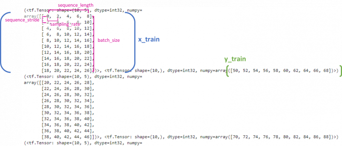
この時、x_train, y_trainは先ほど設定した説明変数、目的変数を入力します。seauence_length, sequence_stride, sampling_rate, batch_sizeについては深層学習に精通している場合はすでに意味が分かっていると思います。わかっていない場合でもこのメソッドの結果を見ればある程度理解できると思います。今回はそれぞれ、以下のように設定しています。
- sequence_length : バッチ内の一つのシーケンス(アレイ)の長さ
- sampling_rate : 元データからサンプリングする間隔。データが間引きされます
- sequence_stride : ストライド、シーケンス間の間隔のような感じ
- batch_size : データをバッチに分けた時の一つのバッチのサイズ
from tensorflow import keras
dataset_train = keras.preprocessing.timeseries_dataset_from_array(
    x_train,
    y_train,
    sequence_length=5,
    sequence_stride=2,
    sampling_rate=2,
    batch_size=10,
)
結果を確認
では、次にメソッドの出力を確認していきます。
print('len_dataset_train:',len(dataset_train))
for batch in dataset_train:
    print(batch)
結果
len_dataset_train: 8
(<tf.Tensor: shape=(10, 5), dtype=int32, numpy=
array([[ 0,  2,  4,  6,  8],
       [ 2,  4,  6,  8, 10],
       [ 4,  6,  8, 10, 12],
       [ 6,  8, 10, 12, 14],
       [ 8, 10, 12, 14, 16],
       [10, 12, 14, 16, 18],
       [12, 14, 16, 18, 20],
       [14, 16, 18, 20, 22],
       [16, 18, 20, 22, 24],
       [18, 20, 22, 24, 26]])>, <tf.Tensor: shape=(10,), dtype=int32, numpy=array([50, 52, 54, 56, 58, 60, 62, 64, 66, 68])>)
(<tf.Tensor: shape=(10, 5), dtype=int32, numpy=
array([[20, 22, 24, 26, 28],
       [22, 24, 26, 28, 30],
       [24, 26, 28, 30, 32],
       [26, 28, 30, 32, 34],
       [28, 30, 32, 34, 36],
       [30, 32, 34, 36, 38],
       [32, 34, 36, 38, 40],
       [34, 36, 38, 40, 42],
       [36, 38, 40, 42, 44],
       [38, 40, 42, 44, 46]])>, <tf.Tensor: shape=(10,), dtype=int32, numpy=array([70, 72, 74, 76, 78, 80, 82, 84, 86, 88])>)
(<tf.Tensor: shape=(10, 5), dtype=int32, numpy=
array([[40, 42, 44, 46, 48],
       [42, 44, 46, 48, 50],
       [44, 46, 48, 50, 52],
       [46, 48, 50, 52, 54],
       [48, 50, 52, 54, 56],
       [50, 52, 54, 56, 58],
       [52, 54, 56, 58, 60],
       [54, 56, 58, 60, 62],
       [56, 58, 60, 62, 64],
       [58, 60, 62, 64, 66]])>, <tf.Tensor: shape=(10,), dtype=int32, numpy=array([ 90,  92,  94,  96,  98, 100, 102, 104, 106, 108])>)
(<tf.Tensor: shape=(10, 5), dtype=int32, numpy=
array([[60, 62, 64, 66, 68],
       [62, 64, 66, 68, 70],
       [64, 66, 68, 70, 72],
       [66, 68, 70, 72, 74],
       [68, 70, 72, 74, 76],
       [70, 72, 74, 76, 78],
       [72, 74, 76, 78, 80],
       [74, 76, 78, 80, 82],
       [76, 78, 80, 82, 84],
       [78, 80, 82, 84, 86]])>, <tf.Tensor: shape=(10,), dtype=int32, numpy=array([110, 112, 114, 116, 118, 120, 122, 124, 126, 128])>)
(<tf.Tensor: shape=(10, 5), dtype=int32, numpy=
array([[ 80,  82,  84,  86,  88],
       [ 82,  84,  86,  88,  90],
       [ 84,  86,  88,  90,  92],
       [ 86,  88,  90,  92,  94],
       [ 88,  90,  92,  94,  96],
       [ 90,  92,  94,  96,  98],
       [ 92,  94,  96,  98, 100],
       [ 94,  96,  98, 100, 102],
       [ 96,  98, 100, 102, 104],
       [ 98, 100, 102, 104, 106]])>, <tf.Tensor: shape=(10,), dtype=int32, numpy=array([130, 132, 134, 136, 138, 140, 142, 144, 146, 148])>)
(<tf.Tensor: shape=(10, 5), dtype=int32, numpy=
array([[100, 102, 104, 106, 108],
       [102, 104, 106, 108, 110],
       [104, 106, 108, 110, 112],
       [106, 108, 110, 112, 114],
       [108, 110, 112, 114, 116],
       [110, 112, 114, 116, 118],
       [112, 114, 116, 118, 120],
       [114, 116, 118, 120, 122],
       [116, 118, 120, 122, 124],
       [118, 120, 122, 124, 126]])>, <tf.Tensor: shape=(10,), dtype=int32, numpy=array([150, 152, 154, 156, 158, 160, 162, 164, 166, 168])>)
(<tf.Tensor: shape=(10, 5), dtype=int32, numpy=
array([[120, 122, 124, 126, 128],
       [122, 124, 126, 128, 130],
       [124, 126, 128, 130, 132],
       [126, 128, 130, 132, 134],
       [128, 130, 132, 134, 136],
       [130, 132, 134, 136, 138],
       [132, 134, 136, 138, 140],
       [134, 136, 138, 140, 142],
       [136, 138, 140, 142, 144],
       [138, 140, 142, 144, 146]])>, <tf.Tensor: shape=(10,), dtype=int32, numpy=array([170, 172, 174, 176, 178, 180, 182, 184, 186, 188])>)
(<tf.Tensor: shape=(1, 5), dtype=int32, numpy=array([[140, 142, 144, 146, 148]])>, <tf.Tensor: shape=(1,), dtype=int32, numpy=array([190])>)
メソッドに設定したパラメータと出力の関係を表すと次のような対応です。
自分で作った配列でメソッドを試すと理解しやすいですね。便利なメソッドなので時系列データについては今後も多用できそうです。